

How to Bake Functions from Scratch?
Ece Paksoy
In physics, to find how a pendulum behaves the equation T(1 - cosx) - x being the angle between the equilibrium position and the rod, and T being the length of the string- is used. However, to help the students solve problems without their calculators, their teacher shows them another equation that looks like and substitutes cosx with . When we plot both functions, they do resemble each other for small angles near zero but how can we even think to find these approximations?
Let’s look at the function cosx and try to find how this approximation works. We will try to find a new polynomial function that resembles the cosx function in which it looks like . At first, since we will approximate according to 0 and since at x = 0 the value of cosx goes to 1, our approximation should pass through the point (0,1). Thus, the constant number of our polynomial will be 1. Even though y = 1 satisfies the x = 0 point, we need to add new layers to make it similar to cosx.

It will also be good that our equation has the same slope as cosx at the point of interest. The derivative of cosx is -sinx and at x=0, it is 0, meaning that there is a horizontal tangent at x=1. Thus, since the first degree derivative of our function at x=0 is 0, we can conclude that the coefficient of x in our polynomial (b) is 0. Nothing changes, and we continue with y=1.
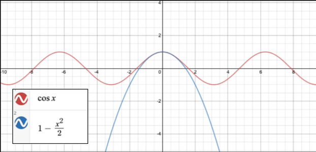
Now, we will try to find some value for c so that our function will curve down just like cosx. We will get the second derivative of cosx, to make sure that its second derivative matches each other. The second derivative of cosx is -cosx while the second derivative of our function is 2c. Since -cos(0) goes to -1, by equalizing 2c to -1 we are able to find the value of c as .
If we want to continue, we can add new layers to our function which will then look like
It’s time to take the third derivative of the functions and equalize them. The third derivative of cosx is sinx which will be equal to the third derivative of our function that is 3.2.1.d + 4.3.2.e.x. When we equalize these functions at x=0, we find the value of d as 0. To find the value of e, we will take the fourth derivative which will be equal to the fourth derivative of cosx which is cosx again. Thus, 4.3.2.1.e becomes equal to cosx at x=0 and e is . When we graph the equation we found as , it will look like the graph below which is a very close approximation of cosx around 0.

We can conclude that
-
Adding new layers to the equation didn’t affect the previous terms since we plug 0 and any higher term will get washed away.
-
While equalizing the coefficients to the derivatives, we divided the desired derivative value to the factorial of the derivatives’ level because of the power rule. For example, while finding the coefficient of , we divided the value by 4!.
-
If instead, we were to approximate a value other than 0 (for example x=pi), in order to get the same effect, we will write our polynomial function with (x-π). Our function will be .
In short, by Taylor’s Theorem, we can find polynomial substitutes for nonpolynomial functions that approximate them near some input. It is formulated as
Theoretically, by adding new terms infinitely, we can find an approximation just the same as the original function.
References:
“Intro to Taylor Series: Approximations on Steroids.” YouTube, 6 Mar. 2019, youtu.be/9YAaCEA08yM.
“Taylor Polynomials.” YouTube, 18 June 2008, youtu.be/8SsC5st4LnI.
“Taylor Series: Essence of Calculus, Chapter 11.” YouTube, 7 May 2017, youtu.be/3d6DsjIBzJ4.